Band Structure
Band structure computations are available on the top of standard workflow SCF/post-SCF molecular computations with the BANDS module. Bands calculations make sense if the molecular structure is an ordered oligomer with insignificant deviations from periodic regularity.
To carry out such calculations, restrictions are introduced on the order of atoms in the initial structure: 1) periodically repeated units are given one by one from the one end of the oligomer to the other; 2) the order of atoms in each unit mast be identical; 3) terminal groups of atoms (normally terminal H atoms) must be numbered last. The keyword ATOM_CELL must be given in the mqcp input file to define the number if atom in the unit cell. Optional keywords EN_LOWER and EN_UPPER can be specified in the input file to define desired energy range (in eV). The input example is the following:
The input example of [C2H2]15 oligomer.
natom=62
6.0      0.305450260       -17.455528492         0.000000000
1.0      1.375447159       -17.458106142         0.000000000
6.0     -0.386647810       -16.250082413         0.000000000
1.0     -1.456644709       -16.247504763         0.000000000
6.0      0.311250090       -15.047984853         0.000000000
...
6.0      0.386647810        16.250082413         0.000000000
1.0      1.456644709        16.247504763         0.000000000
6.0     -0.305450260        17.455528492         0.000000000
1.0     -1.375447159        17.458106142         0.000000000
1.0      0.231780490        18.380884162         0.000000000
1.0     -0.231780490       -18.380884162         0.000000000
charge=0
Hamilton= dft
Basis=6-31G(d)
charge=0
scftype=rhf
runtype=energy
atoms_cell=4
en_lower=-12
en_upper=5
$libxc functional=b3lyp5 $end
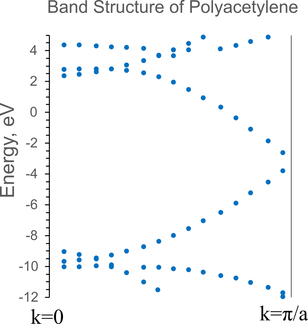
As a result, a table of the dependence of the energy of orbitals on the wave vector is given in the output file. The figure below shows a graphical representation of the dispersion of orbital energies in the Brillouin zone of polyacetylene as the result of calculations.
Dyson’s Orbitals
Quasiparticle states calculations are available with IPDO and EADO modules. The input file is a standard MRSF input with additional options, MREKT=.T. for IPDO and MRDAE=.T. for EADO, in TDDFT section. The particular computation examples are the following.
1. Calculation of Ionization Potentials and Dyson’s Orbitals of based on EKT.
IonizationPotentials presents ionization energies of first 6th Dyson’s orbitals and symmetries of orbital electron distributions calculated for pyridine and thiophene using the functional BH&HLYP with the basis sets 6-311G(d,p).
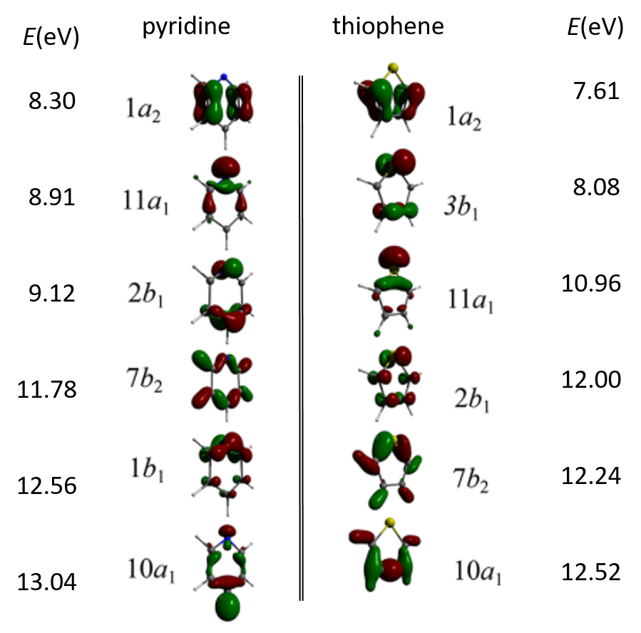
First six Dyson’s HOMOs and the corresponding ionization potentials for the pyridine and thiophene molecules
2. Calculation of Electron Affinities and Dyson’s Orbitals based on EKT.
ElectronAffinities presents energies of electron affinities and orbital electron distributions for Ground (GS) and first excited states S1 of azulene and anthracene calculated using BH&HLYP with the basis sets 6-311G(d,p). Electron occupation corresponds to (1-norm) in parentheses where double is close to 1 and single is about a half.
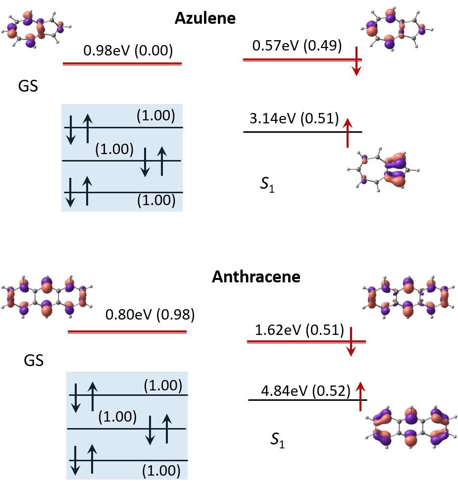
Electronic affinities of azulene and antracene molecules
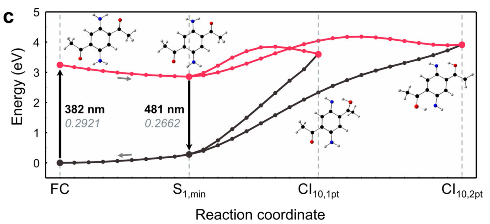
Minimum Energy Path by geodesic interpolation
26
s1fc
C       3.5074247314   0.3939945603   0.9561861839
C       3.7430749260   1.7842751404   0.8448560724
C       2.2261337252  -0.0579432126   0.6663989400
C       1.1840656346   0.7763155739   0.2723400367
C       1.4197493849   2.1665706794   0.1609385874
C       2.7010691216   2.6184919661   0.4506994956
N       4.4929415572  -0.5096377488   1.2756518870
N       0.4342322172   3.0701092111  -0.1585939230
C      -0.1373319954   0.1920310365  -0.0536972344
O      -1.0495946023   0.8670208928  -0.4881352761
C      -0.3615458522  -1.2884341119   0.1482942157
C       5.0646069048   2.3685208639   1.1706703299
O       5.9766508781   1.6937349040   1.6058692066
C       5.2892619238   3.8486101124   0.9671948773
H       2.0490335062  -1.1175514715   0.7382152340
H       2.8781390989   3.6780910695   0.3788567937
H       5.3197918007  -0.1225164745   1.6879206682
H       4.1838944160  -1.3832384608   1.6534377841
H      -0.3927688414   2.6829179836  -0.5705394985
H       0.7432748350   3.9437964192  -0.5362096520
H      -1.3948773182  -1.5070508453  -0.0898719622
H      -0.1567258677  -1.5836908173   1.1740794058
H       0.2849248363  -1.8744653080  -0.5007717299
H       6.3226530998   4.0671439452   1.2050330686
H       4.6432258826   4.4360613603   1.6155557834
H       5.0839659969   4.1428327319  -0.0588392940
26
s1min
C       3.4761900485   0.4269445477   1.0005782683
C       3.7810792620   1.8283788032   0.8640811736
C       2.1990570653  -0.0627847739   0.6962965902
C       1.1464985855   0.7318890499   0.2517597757
C       1.4516080827   2.1332233599   0.1146131197
C       2.7285626812   2.6230763437   0.4194472611
N       4.4351827379  -0.4070644472   1.4237551748
N       0.4928983086   2.9670874961  -0.3093993543
C      -0.1623213857   0.1965618224  -0.0522583917
O      -1.1020148873   0.9007180314  -0.4528085932
C      -0.3988330787  -1.2844624423   0.1254910682
C       5.0895838269   2.3638539859   1.1690337052
O       6.0295679290   1.6596430324   1.5687918298
C       5.3255065354   3.8452995076   0.9934910447
H       2.0427184108  -1.1214526583   0.8203282149
H       2.8847328238   3.6818009713   0.2955286689
H       5.3400891076   0.0019046668   1.6309033353
H       4.2571999553  -1.3856935040   1.5299325718
H      -0.4120348220   2.5582687450  -0.5168667968
H       0.6706893292   3.9457379869  -0.4158557266
H      -1.4321566221  -1.4910584825  -0.1245708569
H      -0.2139476838  -1.6039518689   1.1499509230
H       0.2447709419  -1.8771143289  -0.5232477595
H       6.3585566810   4.0522547842   1.2444582748
H       4.6811311911   4.4366253746   1.6427089996
H       5.1409549758   4.1663039968  -0.0306025204
This is example of xyz file to generate geodesic MEP used in Nat Commun 12, 5409 (2021).
To generate geodesic MEP, one has to create xyz file that contains two geometries (starting / end points)
Nucleus Independent Chemical Shift (NICS) calculation using Dalton Package
### dal input
**DALTON INPUT
.RUN PROPERTIES
**WAVE FUNCTION
.HF
.MCSCF
*CONFIGURATION INPUT
.SYMMETRY
1
.SPIN MULTIPLICITY
1
.INACTIVE
50
.CAS SPACE
2
.ELECTRONS
2
*OPTIMIZATION
.STATE
2
**PROPERTIES
.SHIELD
**END OF DALTON INPUT


### mol input
ATOMBASIS
p-DAPA
comment
Atomtypes=5 NoSymmetry
Charge=8.0 Atoms=2 Basis=6-31G*
O        6.842672938     -1.322637495     -0.162989887
O       -6.842806547      1.322426516      0.164581259
Charge=7.0 Atoms=2 Basis=6-31G*
N       -2.873078816      4.437821733     -0.186528694
N        2.873188598     -4.437720436      0.186773595
Charge=6.0 Atoms=10 Basis=6-31G*
C       -1.509342993      2.231853428     -0.035812371
C       -2.647694531     -0.186634704     -0.027091463
C        1.114090031      2.323111837     -0.001476878
C        2.647736711      0.186558340      0.027630884
C        1.509371237     -2.231894884      0.036199806
C       -1.114091660     -2.323119957      0.001798048
C        5.430726067      0.482124954     -0.014101475
C        6.560085910      3.101394554      0.113080808
C       -5.430801807     -0.482151274      0.014160237
C       -6.560086713     -3.101092723     -0.116013825
Charge=1.0 Atoms=12 Basis=6-31G*
H        1.982920439      4.162690998     -0.032902303
H       -1.982852555     -4.162706982      0.033189390
H       -4.716232184      4.292201888      0.219892747
H       -2.008141452      5.995991523      0.445999286
H        4.716506059     -4.291926296     -0.219004079
H        2.008137723     -5.995983626     -0.445424854
H        8.596643166      2.912195785      0.167509737
H        5.922869022      4.110825239      1.784525572
H        6.031880619      4.215477089     -1.531034553
H       -8.596561221     -2.911839727     -0.171084349
H       -6.033129431     -4.217774292      1.526944615
H       -5.921352775     -4.108991587     -1.787906959
Charge=0.0 Atoms=5 Basis=pointcharge
X        0.000021090     -0.000038182      0.000000000
X        0.000021090     -0.000038182      0.944862994
X        0.000021090     -0.000038182      1.889725989
X        0.000021090     -0.000038182      3.779451977
X        0.000021090     -0.000038182      5.669177966
This is NICS calculation on top of CASSCF(2,2)/6-31G* wavefunction used in Nat Commun 12, 5409 (2021).
Note that Dalton requires two inputs (input.dal / input.mol).
We calculate NICS values using ghost atoms (X) that are put above the center of benzene ring (0, 0.5, 1.0, 2.0, 3.0 Angstrom).

Maximum Overlap Method (MOM) calculation
$CONTRL  SCFTYP=ROHF RUNTYP=ENERGY DFTTYP=BP86 ICHARG=1
TDDFT=MRSF MAXIT=200 MULT=3 ISPHER=1  $END
$TDDFT  NSTATE=8 IROOT=1 MULT=1  $END
$SCF  DIRSCF=.T. diis=.t. soscf=.f. damp=.t. shift=.t.
swdiis=1e-4 mom=.t.  $END
$BASIS  GBASIS=SPK-DZP  $END
$SYSTEM  TIMLIM=999999100 MWORDS=500  $END
$GUESS  guess=moread norb=586  $END
$DFT DFTTYP=BP86 swoff=1e-6 sg1=.t. NRAD0=50 NLEB0=110 $END
$DATA
MeCbl 2.00
C1
N  7.0   -0.0624430   -0.1132311    1.7483714
Co 27.0  -0.0061051    0.0164836   -0.4207477
C  6.0   -3.2784169   -0.1968389   -0.4357658
C  6.0   -0.0480683    0.1521549   -2.4156871
H  1.0    0.3963554    1.1102324   -2.7139713
H  1.0    0.5126009   -0.6847181   -2.8508229
H  1.0   -1.0991660    0.1044608   -2.7278236
H  1.0   -4.3662141   -0.2693960   -0.4385652
C  6.0   -2.5657964   -1.3936154   -0.4756937
C  6.0   -3.2295671   -2.7497398   -0.5028914
C  6.0   -2.7304937    1.0827493   -0.4201847
C  6.0   -3.5612378    2.3438803   -0.4288008
N  7.0   -1.2167798   -1.4938324   -0.4945363
N  7.0   -1.4047733    1.3581454   -0.4000123
C  6.0   -0.8316992   -2.8219770   -0.5260048
C  6.0   -2.0444940   -3.7267350   -0.5348367
C  6.0   -1.1959306    2.7224982   -0.4943585
C  6.0   -2.5151505    3.4527244   -0.6185229
C  6.0    0.4657791   -3.2769236   -0.5319828
H  1.0    0.6330652   -4.3534559   -0.5386831
C  6.0    0.0311018    3.3424730   -0.4891331
H  1.0    0.0596883    4.4279750   -0.5769618
C  6.0    1.5975802   -2.4173960   -0.5539798
C  6.0    3.0481635   -2.8466095   -0.6310661
C  6.0    1.2614677    2.6434512   -0.3505205
C  6.0    2.6358480    3.2684188   -0.2365601
N  7.0    1.4890249   -1.1132326   -0.5421504
C  6.0    2.8023916   -0.4595798   -0.7444275
N  7.0    1.3213202    1.3394639   -0.2641629
C  6.0    2.7024681    0.8684759   -0.0062929
C  6.0    0.0790660   -1.2325912    2.5477945
H  1.0    0.2458472   -2.2172693    2.1261106
C  6.0   -0.0266652   -0.8707181    3.8706666
H  1.0    0.0256305   -1.4424043    4.7896892
N  7.0   -0.2341697    0.4910496    3.8646645
H  1.0   -0.3556976    1.0818008    4.6823436
C  6.0   -0.2494666    0.9121245    2.5755304
H  1.0   -0.3961902    1.9478540    2.2904586
C  6.0    3.8036821   -1.5364699   -0.3063101
C  6.0    3.5758765    2.0568291   -0.4362581
H  1.0    2.9104427   -0.2457789   -1.8249529
H  1.0    2.7981622    0.6753905    1.0784427
H  1.0    3.8415539    1.9573456   -1.4995035
H  1.0    4.5028482    2.1339770    0.1439416
H  1.0   -3.8704695   -2.8826991    0.3807287
H  1.0    2.7862550    4.0687539   -0.9735636
H  1.0   -2.5903115    3.9200573   -1.6117427
H  1.0    2.7552589    3.7222912    0.7614094
H  1.0   -4.3186871    2.3171427   -1.2235215
H  1.0    3.9829582   -1.4613543    0.7769532
H  1.0    4.7676256   -1.4579825   -0.8226923
H  1.0    3.2737546   -3.2072263   -1.6488382
H  1.0    3.2736080   -3.6702306    0.0595988
H  1.0   -2.5958611    4.2599996    0.1211719
H  1.0   -2.0432622   -4.3609201   -1.4323997
H  1.0   -4.1031145    2.4414718    0.5246480
H  1.0   -2.0293491   -4.4021608    0.3318621
H  1.0   -3.8822994   -2.8415614   -1.3831333
$END
--- OPEN SHELL ORBITALS --- GENERATED AT Tue Mar  9 13:41:44 2021
Ref orbital at 1.85
E(RO-BP86)=    -2604.7250403089, E(NUC)= 3915.3398553345,  100 ITERS
$VEC
~~~
$END
This is example input of using MOM. This method can be used when you want to use specific reference orbital given in
$VEC.
LR-TDDFT calculation
$CONTRL  SCFTYP=RHF RUNTYP=ENERGY DFTTYP=B3LYP ICHARG=0
TDDFT=EXCITE MAXIT=200 MULT=1 ISPHER=1 $END
$TDDFT  NSTATE=6 MULT=1  $END
$SCF  DIRSCF=.T. DIIS=.T.  $END
$BASIS  GBASIS=CCT  $END
$SYSTEM  TIMLIM=999999100 MWORDS=500  $END
$DATA
Butadiene TDDFT
Cnh 2

C        6.0     -0.410990219    -1.798958603    0.000000000
C        6.0     -0.559475119    -0.470573512    0.000000000
H        1.0     -1.263114858    -2.463113554    0.000000000
H        1.0     -1.554995711    -0.040726039    0.000000000
H        1.0     -0.571968115    2.252448386     0.000000000
$END
This is LR-TDDFT/B3LYP input for butadiene used in J. Phys. Chem. Lett. 2021, 12, 9720-9729
Delta-CR-EOMCC(2,3) calculation
$CONTRL SCFTYP=RHF RUNTYP=ENERGY ICHARG=0 CCTYP=CR-EOML
MAXIT=200 MULT=1 ISPHER=1 NUMGRD=.T. $END
$SCF  DIRSCF=.T. DIIS=.T.   $END
$BASIS  GBASIS=CCT  $END
$SYSTEM  TIMLIM=999999100 MWORDS=1000  $END
$EOMINP  nstate(1)=2,0,0,1 MTRIP=4  $END
$DATA
Buta delta-CR-EOMCC(2,3)
Cnh 2

C     6.0     -0.410990219    -1.798958603    0.000000000
C     6.0     -0.559475119    -0.470573512    0.000000000
H     1.0     -1.263114858    -2.463113554    0.000000000
H     1.0     -1.554995711    -0.040726039    0.000000000
H     1.0     0.571968115     -2.252448386    0.000000000
$END
This is delta-CR-EOMCC(2,3) input for butadiene used in J. Phys. Chem. Lett. 2021, 12, 9720-9729
CASSCF calculation
$CONTRL  SCFTYP=MCSCF RUNTYP=ENERGY ICHARG=0
MAXIT=200 MULT=1 ISPHER=1 MPLEVL=2 $END
$SCF  DIRSCF=.T. DIIS=.T.  $END
$BASIS  GBASIS=CCT  $END
$SYSTEM  TIMLIM=999999100 MWORDS=1000 $END
$GUESS  GUESS=MOREAD NORB=17 NORDER=1 IORDER(13)=14,13,15,16,17  $END
$MCSCF  CISTEP=ALDET FOCAS=.F. SOSCF=.T. MAXIT=200  $END
$DET  GROUP=C2H STSYM=BU
NCORE=13 NACT=4 NELS=4 NSTATE=10 WSTATE(1)=1,1  $END
$DATA
Butadiene CASSCF(4.4)
Cnh 2

C        6.0     -0.410990219    -1.798958603    0.000000000
C        6.0     -0.559475119    -0.470573512    0.000000000
H        1.0     -1.263114858    -2.463113554    0.000000000
H        1.0     -1.554995711    -0.040726039    0.000000000
H        1.0     -0.571968115    2.252448386     0.000000000
$END
--- NATURAL ORBITALS OF MCSCF --- GENERATED AT 21:17:43 13-MAY-2021
Orbital at FC geometry
E(MCSCF)=     -154.9954698060, E(NUC)=      103.8314056120
$VEC
~~~
$END
This is CASSCF(4,4) input for butadiene used in J. Phys. Chem. Lett. 2021, 12, 9720-9729
We calculate 2 state average CASSCF of Bu state of butadiene in C2h symmetry.
Note that we reordered initial orbital.
XMCQDPT2 calculation
$CONTRL  SCFTYP=MCSCF RUNTYP=ENERGY ICHARG=0
MAXIT=200 MULT=1 ISPHER=1 MPLEVL=2 $END
$SCF  DIRSCF=.T. DIIS=.T.  $END
$BASIS  GBASIS=CCT  $END
$SYSTEM  TIMLIM=999999100 MWORDS=1000 $END
$GUESS  GUESS=MOREAD NORB=17 NORDER=1 IORDER(13)=14,13,15,16,17  $END
$MCSCF  CISTEP=ALDET FOCAS=.F. SOSCF=.T. MAXIT=200  $END
$DET  GROUP=C2H STSYM=BU
NCORE=13 NACT=4 NELS=4 NSTATE=10 WSTATE(1)=1,1  $END
$MRMP MRPT=MCQDPT $END
$MCQDPT  STSYM=BU NSTATE=10 KSTATE(1)=1,1 WSTATE(1)=1,1
XZERO=.T. $END
$DATA
Butadiene XMCQDPT2(4.4)
Cnh 2

C        6.0     -0.410990219    -1.798958603    0.000000000
C        6.0     -0.559475119    -0.470573512    0.000000000
H        1.0     -1.263114858    -2.463113554    0.000000000
H        1.0     -1.554995711    -0.040726039    0.000000000
H        1.0     -0.571968115    2.252448386     0.000000000
$END
--- NATURAL ORBITALS OF MCSCF --- GENERATED AT 21:17:43 13-MAY-2021
Orbital at FC geometry
E(MCSCF)=     -154.9954698060, E(NUC)=      103.8314056120
$VEC
~~~
$END
This is XMCQDPT2(4,4) input for butadiene used in J. Phys. Chem. Lett. 2021, 12, 9720−9729
Note that we reordered initial orbital.
MRMP2 calculation
$CONTRL  SCFTYP=MCSCF RUNTYP=ENERGY ICHARG=0
MAXIT=200 MULT=1 ISPHER=1 MPLEVL=2 $END
$SCF  DIRSCF=.T. DIIS=.T.  $END
$BASIS  GBASIS=CCT  $END
$SYSTEM  TIMLIM=999999100 MWORDS=1000 $END
$GUESS  GUESS=MOREAD NORB=17 NORDER=1 IORDER(13)=14,13,15,16,17  $END
$MCSCF  CISTEP=ALDET FOCAS=.F. SOSCF=.T. MAXIT=200  $END
$DET  GROUP=C2H STSYM=BU
NCORE=13 NACT=4 NELS=4 NSTATE=10 WSTATE(1)=1,1  $END
$MRMP MRPT=MCQDPT $END
$MCQDPT  STSYM=Bu NSTATE=10 KSTATE(1)=1,0 WSTATE(1)=1,0
XZERO=.F.  $END
$DATA
Butadiene MRMP2
Cnh 2

C        6.0     -0.410990219    -1.798958603    0.000000000
C        6.0     -0.559475119    -0.470573512    0.000000000
H        1.0     -1.263114858    -2.463113554    0.000000000
H        1.0     -1.554995711    -0.040726039    0.000000000
H        1.0     -0.571968115    2.252448386     0.000000000
$END
--- NATURAL ORBITALS OF MCSCF --- GENERATED AT 21:17:43 13-MAY-2021
Orbital at FC geometry
E(MCSCF)=     -154.9954698060, E(NUC)=      103.8314056120
$VEC
~~~
$END
This is MRMP2 input for butadiene used in J. Phys. Chem. Lett. 2021, 12, 9720-9729
Note that we reordered initial orbital.
Conical Intersection optimization
 $CONTRL  SCFTYP=ROHF RUNTYP=CONICAL DFTTYP=BHHLYP ICHARG=0
 TDDFT=MRSF MAXIT=200 MULT=3 $END
 $CONICL  IXROOT(1)=1,2 $END
 $TDDFT   NSTATE=3 IROOT=2 MULT=1 $END
 $SCF     DIRSCF=.T. DIIS=.T.  $END
 $BASIS   GBASIS=N31 NGAUSS=6 NDFUNC=1 $END
 $STATPT  NSTEP=150 $END
 $SYSTEM  TIMLIM=999999100 MWORDS=500  $END
 $DATA
Thymine CI10 optimization
C1
C           6.0  -6.3694490194   3.3066040959   0.6701853348
C           6.0  -5.1383739860   2.5156794815   0.3450907496
C           6.0  -5.2128492716   1.0973250281   0.5420397967
C           6.0  -7.4147564086   1.5675884803  -0.5727641378
C           6.0  -3.9774834523   3.2436330141  -0.2019998520
N           7.0  -6.1240564597   1.0691991511  -0.6096436795
N           7.0  -7.5125831049   2.6034163480   0.3503600316
O           8.0  -8.3186768725   1.1989581009  -1.2681645527
O           8.0  -6.3549614051   4.3990557850   1.1739453250
H           1.0  -5.9018654502   0.5164108991  -1.4202506441
H           1.0  -8.4041193810   3.0517186642   0.4596019320
H           1.0  -3.3162568968   2.5573719510  -0.7163454661
H           1.0  -3.4282807909   3.6411117522   0.6581871107
H           1.0  -4.2491229046   4.0903025662  -0.8242064803
H           1.0  -5.6839825963   0.7285646824   1.4439495321
 $END
This is input for optimization of conical intersection (CI) used in J.Chem.Phys.Lett.(2021), 12, 4339.
We optimized CI0/1 (ground state / first excited state) of thymine molecule with MRSF-TDDFT/BH&HLYP/6-31G* method. (
IXROOT(1)=1,2)

Non-adiabatic molecular dynamics (NAMD) simulaion
 $CONTRL  SCFTYP=ROHF RUNTYP=MD DFTTYP=BHHLYP ICHARG=0
 TDDFT=MRSF MAXIT=200 MULT=3 UNITS=BOHR  $END
 $TDDFT   NSTATE=3 IROOT=3 MULT=1 $END
 $SCF     DIRSCF=.T. DIIS=.T. $END
 $BASIS   GBASIS=N31 NGAUSS=6 NDFUNC=1 $END
 $SYSTEM  TIMLIM=999999100 MWORDS=500 $END
 $DATA
Thymine NAMD simulation
C1
C     6.0   -11.8505071     6.5206747    -0.0300030
C     6.0    -9.5107081     5.0382484     0.0296647
C     6.0    -9.7175136     2.4272968     0.1217397
C     6.0   -14.2404466     2.2839256    -0.0366132
C     6.0    -7.0401877     6.4071584    -0.3197621
N     7.0   -11.9358493     1.2290798     0.2578589
N     7.0   -14.1275838     4.9013071     0.0834579
O     8.0   -16.1954657     1.2417354    -0.2958192
O     8.0   -12.1015559     8.7906497     0.1551644
H     1.0   -12.0940252    -0.7267109     0.7216047
H     1.0   -15.6585341     5.3990041     0.2736094
H     1.0    -5.4516499     4.9448097    -0.0114726
H     1.0    -6.9028034     7.5913218     1.4849747
H     1.0    -6.8090855     8.1187178    -2.0100609
H     1.0    -8.2001318     1.1305770    -0.1053907
 $END
 $MD  READ=.F. MBT=.T. MBR=.T.
 TTOTAL=0 DT=5e-16 NSTEPS=4000 MDINT=VVERLET
 NVTNH=0 BATHT(1)=300.0 RSTEMP=.F. JEVERY=1 KEVERY=1
 THRSHE=10 NAMD=.T.  $END
This is input for NAMD simulation used in J.Chem.Phys.Lett.(2021), 12, 4339.
We simulate thymine molecule with MRSF-TDDFT/BH&HLYP/6-31G* method.
We excited thymine to bright S2 state (IROOT=3) and propagate it until 2 ps with 0.5 fs timestep. (DT = 0.5 fs, NSTEPS=4000 –> total 2 ps)
* Note that we block the hopping which has greater energy gap between electronic state than 10 kcal/mol (THRSHE=10)
* Note that one can geometry and velocity obtained from Wigner sampling with READ=.T. and TVELQM(1)= 3N values of velocity in atomic unit in MD group.


Singlet Ground State Optimization
 $CONTRL  SCFTYP=ROHF RUNTYP=OPTIMIZE DFTTYP=BHHLYP ICHARG=0
 TDDFT=MRSF MAXIT=200 MULT=3  $END
 $TDDFT   NSTATE=5 IROOT=1 MULT=1 $END
 $SCF     DIRSCF=.T. DIIS=.T. $END
 $BASIS   GBASIS=CCT $END
 $SYSTEM  TIMLIM=999999100 MWORDS=500 $END
 $DATA
O-Benzyne
C1
H           1.0   2.5147391212  -0.0000000000  -0.1133955920
C           6.0   1.4425296188  -0.0000000000  -0.1119841121
C           6.0   0.6976318813  -0.0000000000   1.0655138930
H           1.0   1.2156127180  -0.0000000000   2.0075731367
C           6.0  -0.6976162877  -0.0000000000   1.0655155622
H           1.0  -1.2156221862   0.0000000000   2.0075631596
C           6.0  -1.4425256576   0.0000000000  -0.1119742488
H           1.0  -2.5147353494  -0.0000000000  -0.1134027300
C           6.0  -0.6195526066  -0.0000000000  -1.2085042416
C           6.0   0.6195387483   0.0000000000  -1.2085068269
 $END
Above is the input for Singlet Ground state optimization used in J. Chem. Theory Comput. 2021, 17, 2, 848-859.
We simulated o-benzyne diradical with MRSF-TDDFT/BH&HLYP/cc-pVTZ method.
One ground state singlet and four lowest singlet states are calculated (NSTATE = 5).
Triplet Ground State Optimization
 $CONTRL  SCFTYP=ROHF RUNTYP=OPTIMIZE DFTTYP=BHHLYP ICHARG=0
 TDDFT=MRSF MAXIT=200 MULT=3  $END
 $TDDFT   NSTATE=5 IROOT=1 MULT=3 $END
 $SCF     DIRSCF=.T. DIIS=.T. $END
 $BASIS   GBASIS=CCT $END
 $SYSTEM  TIMLIM=999999100 MWORDS=500 $END
 $DATA
O-Benzyne
C1
HYDROGEN    1.0   2.5147391212  -0.0000000000  -0.1133955920
CARBON      6.0   1.4425296188  -0.0000000000  -0.1119841121
CARBON      6.0   0.6976318813  -0.0000000000   1.0655138930
HYDROGEN    1.0   1.2156127180  -0.0000000000   2.0075731367
CARBON      6.0  -0.6976162877  -0.0000000000   1.0655155622
HYDROGEN    1.0  -1.2156221862   0.0000000000   2.0075631596
CARBON      6.0  -1.4425256576   0.0000000000  -0.1119742488
HYDROGEN    1.0  -2.5147353494  -0.0000000000  -0.1134027300
CARBON      6.0  -0.6195526066  -0.0000000000  -1.2085042416
CARBON      6.0   0.6195387483   0.0000000000  -1.2085068269
 $END
Above is the input for Triplet Ground state optimization used in J. Chem. Theory Comput. 2021, 17, 2, 848-859.
We simulated o-benzyne diradical with MRSF-TDDFT/BH&HLYP/cc-pVTZ method.
One Triplet Ground state and four triplet lowest states are calculated (NSTATE = 5).
The above 2 inputs, singlet ground state (S0) optimization and triplet ground state (T0) optimizations are used for calculating singlet-triplet (ST) gap of diradicals and diradicaloids.

Singlet Ground State Optimization Imposing C2V Symmetry
 $CONTRL  SCFTYP=ROHF RUNTYP=OPTIMIZE DFTTYP=BHHLYP ICHARG=0
 TDDFT=MRSF MAXIT=200 MULT=3  $END
 $TDDFT   NSTATE=5 IROOT=1 MULT=1 $END
 $SCF     DIRSCF=.T. DIIS=.T. $END
 $BASIS   GBASIS=CCT $END
 $SYSTEM  TIMLIM=999999100 MWORDS=500 $END
 $DATA
C4H6
CnV   2

CARBON      6.0      0.000000000         0.000000000        -0.036668884
CARBON      6.0     -1.203065556         0.000000000        -0.711856855
CARBON      6.0      0.000000000         0.000000000         1.456105051
HYDROGEN    1.0     -2.138811217         0.000000000        -0.189475446
HYDROGEN    1.0     -1.230113805         0.000000000        -1.784658245
HYDROGEN    1.0      0.000000000         0.921362405         1.999599679
 $END
Above is the input for Singlet Ground state optimization by imposing C2V symmetry used in J. Chem. Theory Comput. 2021, 17, 2, 848-859.
We Simulated Trimethylenemethane (TMM) with MRSF-TDDFT/BH&HLYP/cc-pVTZ method.
One Ground state singlet and four lowest singlet states are calculated (NSTATE = 5).
In $TDDFT MULT=1 denote singlet.
Triplet Ground State Optimization Imposing C2V Symmetry
 $CONTRL  SCFTYP=ROHF RUNTYP=OPTIMIZE DFTTYP=BHHLYP ICHARG=0
 TDDFT=MRSF MAXIT=200 MULT=3  $END
 $TDDFT   NSTATE=5 IROOT=1 MULT=1 $END
 $SCF     DIRSCF=.T. DIIS=.T. $END
 $BASIS   GBASIS=CCT $END
 $SYSTEM  TIMLIM=999999100 MWORDS=500 $END
 $DATA
C4H6
CnV   2

CARBON      6.0      0.000000000         0.000000000        -0.036668884
CARBON      6.0     -1.203065556         0.000000000        -0.711856855
CARBON      6.0      0.000000000         0.000000000         1.456105051
HYDROGEN    1.0     -2.138811217         0.000000000        -0.189475446
HYDROGEN    1.0     -1.230113805         0.000000000        -1.784658245
HYDROGEN    1.0      0.000000000         0.921362405         1.999599679
 $END
Above is the input for triplet Ground state optimization by imposing C2V symmetry used in J. Chem. Theory Comput. 2021, 17, 2, 848-859.
Simulation is perform for Trimethylenemethane (TMM) with MRSF-TDDFT/BH&HLYP/cc-pVTZ method.
One triplet Ground state and four lowest triplet states are calculated (NSTATE = 5).
In $TDDFT MULT=3 denote triplet.
Ground State Optimization
 $CONTRL  SCFTYP=ROHF RUNTYP=OPTIMIZE DFTTYP=BHHLYP ICHARG=0
 TDDFT=MRSF MAXIT=200 MULT=3  $END
 $TDDFT   NSTATE=3 IROOT=1 MULT=1 $END
 $SCF     DIRSCF=.T. DIIS=.T. $END
 $BASIS   GBASIS=N31 NGAUSS=6 NDFUNC=1 $END
 $SYSTEM  TIMLIM=999999100 MWORDS=500 $END
 $DATA
Cytosine
C1
NITROGEN    7.0  -0.0086829468   0.0149277828   0.0660559171
NITROGEN    7.0   2.3458590473  -0.0091621139   0.0642813499
NITROGEN    7.0  -1.1420053387  -0.0086754893   2.0332447816
CARBON      6.0   1.1400383399  -0.0038705258  -0.6655768360
CARBON      6.0   2.3947342125  -0.0046455567   1.4100335961
CARBON      6.0   1.2551073430   0.0066010052   2.1253976227
CARBON      6.0   0.0395322993   0.0143876096   1.3718087669
OXYGEN      8.0   1.2032360931  -0.0103502365  -1.8709106973
HYDROGEN    1.0   3.1791336241  -0.0190957823  -0.4919314370
HYDROGEN    1.0   3.3724732459  -0.0122330275   1.8596591445
HYDROGEN    1.0   1.2618461171  -0.0011092818   3.1994280444
HYDROGEN    1.0  -1.1825535621   0.2440758431   2.9990286956
HYDROGEN    1.0  -1.9622049931   0.1464934116   1.4798381607
 $END
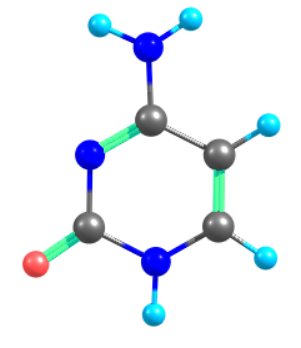
Above is the input for Ground state optimization of Cytosine nucleobase. Simulation is perform for Cytosine Nucleobase using MRSF-TDDFT/BH&HLYP/6-31G(d) method.
Three State Conical Intersection (TCI) Optimization
 $CONTRL  SCFTYP=ROHF RUNTYP=CONICAL DFTTYP=BHHLYP ICHARG=0
 TDDFT=MRSF MAXIT=200 MULT=3  $END
 $TDDFT   NSTATE=4 IROOT=4 MULT=1 TAMMD=.t. $END
 $CONICL  OPTTYP=PENALTT ITROOT(1)=2,3,4 DEBUG=.t. SIGMA=1 $END
 $SCF     DIRSCF=.T. DIIS=.T. $END
 $BASIS   GBASIS=N31 NGAUSS=6 NDFUNC=1 $END
 $STATPT NSTEP=1000 hess=read opttol=1e-10  $END
 $SYSTEM  TIMLIM=999999100 MWORDS=500 $END
 $DATA
Cytosine
C1
NITROGEN    7.0  -0.0086829468   0.0149277828   0.0660559171
NITROGEN    7.0   2.3458590473  -0.0091621139   0.0642813499
NITROGEN    7.0  -1.1420053387  -0.0086754893   2.0332447816
CARBON      6.0   1.1400383399  -0.0038705258  -0.6655768360
CARBON      6.0   2.3947342125  -0.0046455567   1.4100335961
CARBON      6.0   1.2551073430   0.0066010052   2.1253976227
CARBON      6.0   0.0395322993   0.0143876096   1.3718087669
OXYGEN      8.0   1.2032360931  -0.0103502365  -1.8709106973
HYDROGEN    1.0   3.1791336241  -0.0190957823  -0.4919314370
HYDROGEN    1.0   3.3724732459  -0.0122330275   1.8596591445
HYDROGEN    1.0   1.2618461171  -0.0011092818   3.1994280444
HYDROGEN    1.0  -1.1825535621   0.2440758431   2.9990286956
HYDROGEN    1.0  -1.9622049931   0.1464934116   1.4798381607
 $END
 $HESS
 ...
 $END
Above is the input for Three state Conical Intersection optimization of Cytosine nucleobase.
Simulation is perform for Cytosine Nucleobase three state conical intersection using MRSF-TDDFT/BH&HLYP/6-31G(d) method.
ITROOT(1)=2,3,4 is used to locate conical intersection between S1, S2 and S3 excited states.

MRSF-TDDFT Examples using Ethylene
Ethylene S0 optimization
 $CONTRL
  SCFTYP=ROHF RUNTYP=OPTIMIZE DFTTYP=BHHLYP ICHARG=0
  TDDFT=MRSF MAXIT=200 MULT=3
 $END
 $TDDFT
  NSTATE=5 IROOT=1 MULT=1
 $END
 $SCF
  DIRSCF=.T. DIIS=.T. SOSCF=.F.
 $END
 $BASIS
  GBASIS=N31 NGAUSS=6 NDFUNC=1 NPFUNC=1
 $END
 $STATPT NSTEP=250
 $END
 $SYSTEM
  TIMLIM=999999 MWORDS=500
 $END
 $DATA
C2H4 S0 optimization
C1
C    6.0      0.180596175        -0.343800720        -0.175326809
C    6.0      1.465647227        -0.102026293         0.002214204
H    1.0      1.907395230        -0.454760198         0.920551799
H    1.0     -0.127316256         0.024318928        -1.141030591
H    1.0     -0.149587005        -1.321665903         0.137338066
H    1.0      1.822162163         0.910834885        -0.096714838
 $END
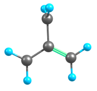
This is input for the ground state optimization of Ethylene with MRSF-TD-DFT/BHH&LYP/6-31G**. Final geometry is shown on the figure below.

Ethylene tw-pyr S1/S0 Conical Intersecrion (CI)
 $CONTRL
  SCFTYP=ROHF RUNTYP=CONICAL DFTTYP=BHHLYP ICHARG=0
  TDDFT=MRSF MAXIT=200 MULT=3
 $END
 $CONICL IXROOT(1)=1,2 $END
 $TDDFT
  NSTATE=5 MULT=1
 $END
 $SCF
  DIRSCF=.T. DIIS=.T. SOSCF=.F.
 $END
 $BASIS
  GBASIS=N31 NGAUSS=6 NDFUNC=1 NPFUNC=1
 $END
 $STATPT NSTEP=250
 $END
 $SYSTEM
  TIMLIM=999999 MWORDS=500
 $END
 $DATA
C2H4 S1/S0 CI
C1
C    6.0    -0.0017163764   0.0292739731  -0.0372180054
C    6.0     1.3786130141   0.0072684726  -0.0080577710
H    1.0     2.0129445494  -0.8878312901   0.0204802061
H    1.0     0.0551578071  -0.6605132877  -0.9497996163
H    1.0    -0.4811626193  -0.7365319361   0.5845879002
H    1.0     1.9748256249   0.9104670683  -0.1296487136
 $END
This is input for the tw-pyr S1/S0 CI optimization of Ethylene (in IXROOT, 1 corresponds to S0, and 2 corresponds to S1 state) with MRSF-TD-DFT/BHH&LYP/6-31G**. The CIs geometry is shown on the figure below.

Ethylene S0 minimum vibrations
 $CONTRL
  SCFTYP=ROHF RUNTYP=HESSIAN DFTTYP=BHHLYP ICHARG=0
  TDDFT=MRSF MAXIT=200 MULT=3
 $END
 $TDDFT
  NSTATE=5 IROOT=1 MULT=1
 $END
 $SCF
  DIRSCF=.T. DIIS=.T. SOSCF=.F.
 $END
 $BASIS
  GBASIS=N31 NGAUSS=6 NDFUNC=1 NPFUNC=1
 $END
 $STATPT NSTEP=250
 $END
 $SYSTEM
  TIMLIM=999999 MWORDS=500
 $END
 $DATA
C2H4 S0 vibrations
C1
CARBON      6.0   0.2737725809  -0.4418423602  -0.2974162841
CARBON      6.0   1.4258439056   0.0128270303   0.1797313338
HYDROGEN    1.0   1.9439319637  -0.4884167117   0.9807203656
HYDROGEN    1.0  -0.2442892276   0.0593372586  -1.0984148091
HYDROGEN    1.0  -0.1906628974  -1.3305950516   0.0969883247
HYDROGEN    1.0   1.8903012088   0.9015905335  -0.2145771000
 $END
This is input for the Ethylene S0 frequency calculations with MRSF-TD-DFT/BHH&LYP/6-31G**
MODE FREQ(CM**-1)  SYMMETRY  RED. MASS  IR INTENS.
  1      18.554    A        1.008760    0.000000
  2       6.650    A        2.121082    0.000000
  3       6.102    A        2.180655    0.000000
  4       0.243    A        4.668636    0.000001
  5       0.065    A        4.672078    0.000000
  6       0.029    A        4.672023    0.000000
  7     860.005    A        1.042244    0.012138
  8    1003.751    A        1.516381    0.000004
  9    1016.337    A        1.160935    2.255860
 10    1116.259    A        1.007826    0.000011
 11    1287.643    A        1.517699    0.000000
 12    1420.859    A        1.271199    0.000000
 13    1531.578    A        1.112140    0.186539
 14    1752.366    A        2.858180    0.000000
 15    3245.587    A        1.047561    0.299122
 16    3262.542    A        1.073808    0.000004
 17    3327.977    A        1.116184    0.000003
 18    3353.094    A        1.118196    0.595658
No imaginary frequencies was obtained
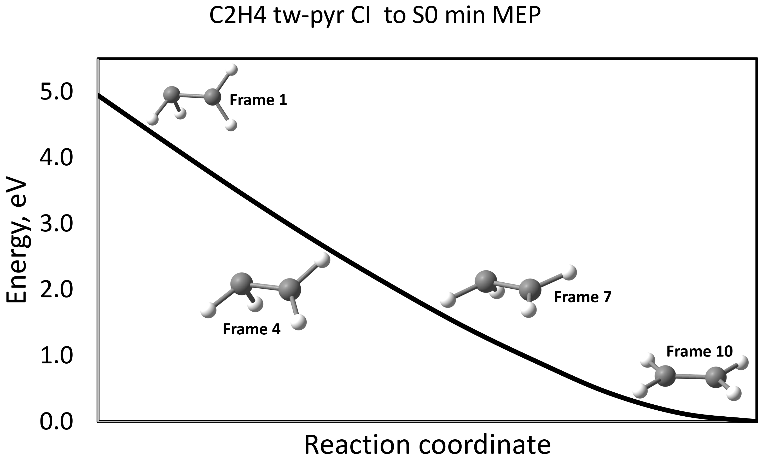
Ethylene {CI (S1/S0) - S0min} MEP using geodesic interpolation
 $CONTRL
  SCFTYP=ROHF RUNTYP=ENERGY DFTTYP=BHHLYP ICHARG=0
  TDDFT=MRSF MAXIT=200 MULT=3
 $END
 $TDDFT
  NSTATE=5 IROOT=1 MULT=1
 $END
 $SCF
  DIRSCF=.T. DIIS=.T.
 $END
 $BASIS
  GBASIS=N31 NGAUSS=6 NDFUNC=1 NPFUNC=1
 $END
 $END
 $SYSTEM
  TIMLIM=999999 MWORDS=500
 $END
 $DATA
C2H4 CI(tw-pyr) - S0min MEP
c1
CARBON      6.0     -0.824885547         0.252330946         0.049317029
CARBON      6.0      0.555605058         0.230100380         0.078834443
HYDROGEN    1.0      1.189859013        -0.665149629         0.106935364
HYDROGEN    1.0     -0.767680817        -0.437452028        -0.863174166
HYDROGEN    1.0     -1.304227831        -0.513413659         0.671248498
HYDROGEN    1.0      1.151330123         1.133583991        -0.043161168
 $END
Here, interpolation between two points on PES was done. For each point (frame) obatined as a result of interpolation, we carried out single point calculations in order to plot the MEP corresponding to the tw-pyr CI - S0min relaxation.