Understanding MRSF-TDDFT Theory
TDDFT
Perhaps, the linear-response (LR)-TDDFT is the most practical formulation of TDDFT, which can be used if the external perturbation is relatively small in the sense that it does not completely destroy the ground-state of a given system. As a result, any variation of the system in the form of responses will depend only on the ground-state wave-function. For example, it simply means that any excited states can be obtained as derived quantities (response states) of ground state, which eliminates the needs for new additional methods to obtain excited states. It should be emphasized that not only exited states but also ground states can be obtained as response states by spin-flip techniques.
Although it has become one of the most popular quantum theories for excited states, there are a number of well-known failures of the popular LR-TDDFT method:
failure to capture non-local properties for long-range charge transfer excited states,
failure to capture double excitation characters in excited states,
poor description of static correlation of the closed-sell reference state undergoing bond breaking
and lack of coupling between the ground and excited states for conical intersections (CI) and avoided crossings.
SF-TDDFT
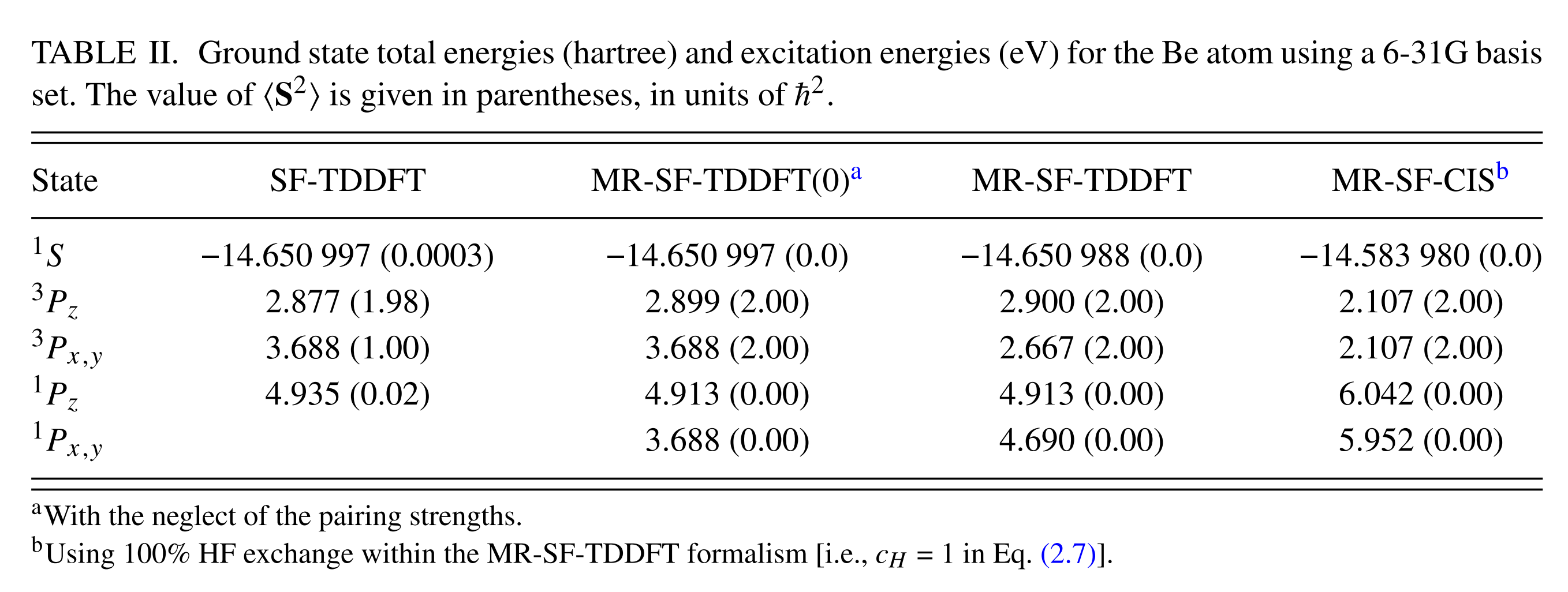
All these drawbacks can be efficiently corrected by the spin-flip (SF)-TDDFT method. It considers an open-shell high-spin triplet state (such as ROHF) as a reference instead of the closed-shell reference of LR-TDDFT. However, the conventional formulation of SF-TDDFT selects only one \(M_S\) = +1 component of the triplet reference (See the figure below), which leads to a considerable spin contamination in the excited states. For example, the state with \(\braket{ S^2}\) = 1.00 in the Be Atom example below represents neither singlet nor triplet state.
The main source of spin contamination comes from the red missing responses (the red configurations below) leading to spin incompleteness. A fundamental solution for this problem is to include red missing configurations in the response space of SF-TDDFT.

Yet another important but not much appreciated source of spin contamiation is from the mismatched contributions of L and R of OO TYPE (the blues). This is because they are coming from different orbitals’ spin-flip transition as shown below. The former and latter comes from spin-flip of O1 and O2 orbitals, respectively. Sometimes, the mismatched contributions introduce a major spin contamination.

MRSF-TDDFT
The red missing configurations can be added into response space by the \(M_S\) = -1 component of ROHF. A hypothetical single reference by combining \(M_S\) = +1 and \(M_S\) = -1 components of ROHF triplet can be constructed by a spinor-like transformation. See more here. The resulting mixed-reference SF-TDDFT (MRSF-TDDFT) eliminates the spin contamination of SF-TDDFT, allowing automatic identification of the electronic states as singlets and triplets. It should be emphasized that MRSF-TDDFT produces not only excited but also ground electronic states. Therefore, open shell singlet such as diradicals, which cannot be studied by the Kohn-Sham DFT, can be naturally described by MRSF-TDDFT.

TDDFT vs. MRSF-TDDFT
There are multiple advantages of MRSF-TDDFT over TDDFT. Here, we list just some of them.
Missing States of C and N+ Atoms
In the case of C and N+ atoms, MRSF-TDDFT produces 8 states of \(^3 P, ^1 D, ^1 S\) as

On the other hand, only 4 states can be represented by TDDFT as
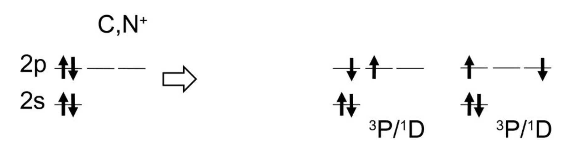
This demonstrates that the conventional TDDFT misses many electronic states. Especially, the doubly excited configuration of \(^1 S\) is completely missing in TDDFT.
Missing States of H2
The \(3 \Sigma_g^{+}\) state (green), entirely composed of doubly excited configuration is missing in TDDFT (LR) but presents in MRSF-TDDFT as shown below in the case of \(H_2\) dissociation.

The doubly excited configuration makes greater contribution to the ground electronic state in the much stretched region, eventually leading to flattening the dissociation curve at the correct dissociation limit shown by the dashed line. On the other hand, the corresponding ground state of LR-PBE0 curve (TDDFT) has to be obtained by DFT, which does not have the correct asymtotic behaviour. See more here.
Curve Crossing of Butadiene
In linear all-trans polyenes, internal conversion (IC) between the \(1^1B{}_u^+\) (optically bright at the Franck-Condon (FC) geometry, the red curve below) and the \(2^1A{}_g^-\) (optically dark, the blues) states has long been argued. However, it hasn’t been proven until recently.
One of the difficulties arising when describing the \(1^1B{}_u^+\) and the \(2^1A{}_g^-\) states is their radically different nature. The former state comprises a one-electron HOMO \(\to\) LUMO transition and it displays pronounced ionic characteristics, while the latter is dominated by HOMO \(\to\) LUMO double excitations, requiring a balanced theory with both dynamic and nondynamic electron correlation.

As seen above, while both MRSF-TDDFT as well as REKS(4,4) produces the right CI as seen in \(\delta\)-CR-EOMCC(2,3), the TDDFT cannot. See more here.
Conical Intersection Topology
Conical Intersection (CI) is a molecular geometry at which two (or more) adiabatic electronic states become degenerate. As the intersecting electronic states at a CI are coupled by the non-vanishing non-adiabatic coupling, CIs provide efficient funnels for the state to state population transfer mediated by the nuclear motion. The degeneracy of the intersecting states at a CI is lifted along two directions in the space of internal molecular coordinates Q, which are defined by the gradient difference and derivative coupling vectors (GDV and DCV, respectively) given by

for the case of a crossing between the ground (\(S_0\)) and the lowest excited \(S_1\) singlet states. The degeneracy is lifted linearly along the GDV and DCV directions, which lends the potential energy surfaces (PESs) of the intersecting states the topology of a double cone below, hence the name. The remaining 3N-8 internal coordinates leave the degeneracy intact, thus defining the crossing seam (or the intersection space) of the CI.
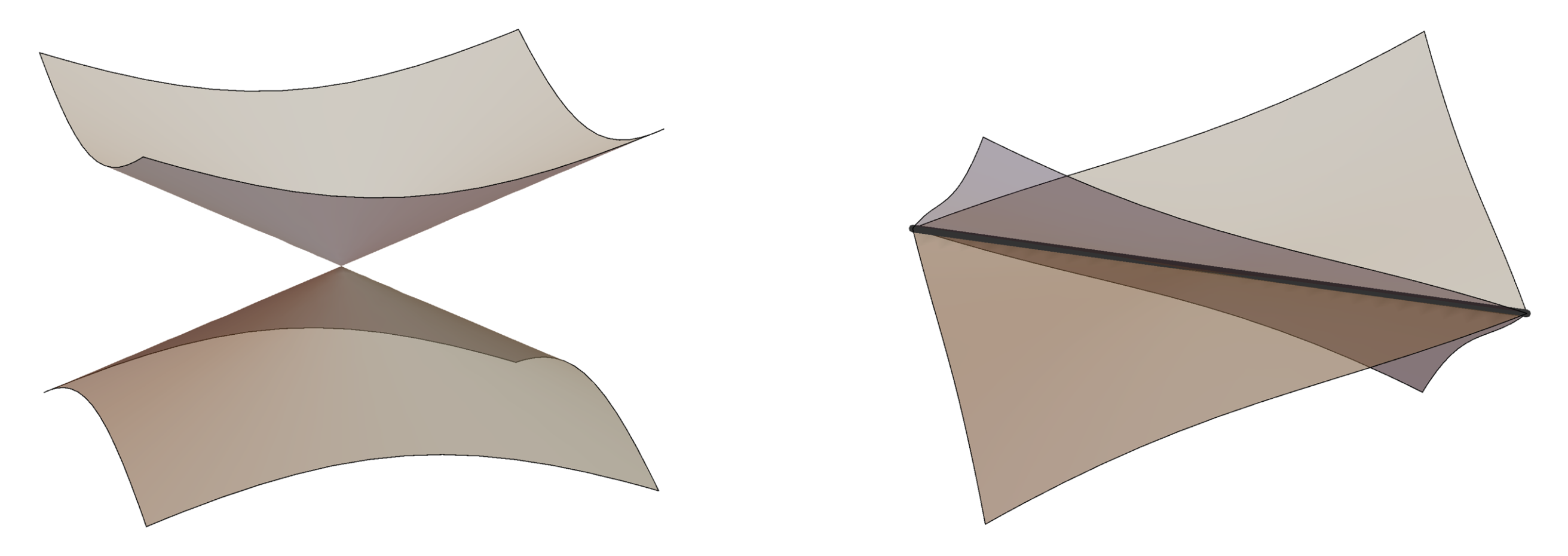
The popular TDDFT fails to yield the correct dimensionality of the CI seam and predicts a linear crossing (3N-7) as shown in the right figure above. The problem is simply rooted in the absence of coupling between the ground (described by reference DFT) and first excited states (described by response of TDDFT).
On the other hand, both ground and first excited states of MRSF-TDDFT are obtained by the same response, producing the correct double cone topology. See more here.
The Reference and Response Triplets
MRSF-TDDFT currently calculates singlet, triplet and quintet states using the ROHF triplet reference. As a result, one may be confused by the two different triplets of reference and responses. Triplet has three states with \(M_s = +1, 0, -1\). Since they are energetically degenerated, nearly all quantum chemistry program calculates the simplest possible state of \(M_s = +1\) as a representative triplet state of ROHF. This particular triplet is the high-spin triplet. On the other hand, the triplet states generated by MRSF-TDDFT are \(M_s = 0\) triplet. Both reference as well as lowest response triplets are supposed to describe the same lowest triplet states with just different \(M_s\). However, their energies are not degenerated. This is because the reference triplet is variationally obtained, while the response triplet is calculated by linear response theory. When you use MRSF-TDDFT, it is always better not to utilize the reference triplet in your analysis.
The Be Atom Case
This simple example can explain a great deal of MRSF-TDDFT calculations. The input example of MRSF-TDDFT with BHHLYP/6-31G basis set for GAMESS is
$CONTRL SCFTYP=ROHF RUNTYP=ENERGY DFTTYP=BHHLYP TDDFT=MRSF MULT=3 $END
$TDDFT  NSTATE=5 IROOT=1 MULT=1 $END
$BASIS  GBASIS=N31 NGAUSS=6 $END
$SCF    DIRSCF=.T. $END
$GUESS  GUESS=HCORE $END
$DATA
Be
C1
BERYLLIUM   4.0     0.0      0.0      0.0
$END
The important keywords are
TDDFT=MRSF : Specifying MRSF-TDDFT method
NSTATE=5 : Total number of excited state requested
IROOT=1 : The target state. For example, the particular state for further geometry optimization.
MULT=3 and =1 : MULT specifies spin multiplicity. Singlet and triplet are 1 and 3, respectively. As you can see, there are 2 different places of MULT. The one in $CONTRL group specifies the spin multiplicity of reference wavefunction. In this case, the ROHF reference state. The MULT in $TDDFT group specifies the spin multiplicity of response states, which are the ones generated by MRSF-TDDFT theory.
This input will prints out the SCF procedures of
ITER EX      TOTAL ENERGY        E CHANGE  DENSITY CHANGE    DIIS ERROR      INTEGRALS    SKIPPED
  1  0      -14.2683005477   -14.2683005477   1.320748431   0.000000000            213          0
  2  1      -14.4986108029    -0.2303102552   0.182168555   0.000000000            213          0
  3  2      -14.5065330145    -0.0079222116   0.012352910   0.000000000            213          0
  4  3      -14.5065504739    -0.0000174594   0.000562434   0.000000000            213          0
CONVERGED TO SWOFF, SO DFT CALCULATION IS NOW SWITCHED ON.
  5  4      -14.5662398400    -0.0596893661   0.035506584   0.000000000            213          0
  6  5      -14.5666215197    -0.0003816797   0.004443966   0.000000000            213          0
  7  6      -14.5666251825    -0.0000036628   0.000788830   0.000000000            213          0
  8  7      -14.5666253040    -0.0000001215   0.000145036   0.000000000            213          0
DFT CODE IS SWITCHING BACK TO THE FINE GRID
  9  8      -14.5666031723     0.0000221317   0.000694477   0.000000000            213          0
 10  9      -14.5666032709    -0.0000000986   0.000133009   0.000000000            213          0
 11 10      -14.5666032742    -0.0000000033   0.000027388   0.000000000            213          0
 12 11      -14.5666032743    -0.0000000001   0.000006101   0.000000000            213          0
 13 12      -14.5666032744    -0.0000000000   0.000003515   0.000000000            213          0
 14 13      -14.5666032744    -0.0000000000   0.000003071   0.000000000            213          0

         ----------------
         ENERGY CONVERGED
         ----------------
    TIME TO FORM FOCK OPERATORS=       0.0 SECONDS (       0.0 SEC/ITER)
    FOCK TIME ON FIRST ITERATION=       0.0, LAST ITERATION=       0.0
    TIME TO SOLVE SCF EQUATIONS=       0.0 SECONDS (       0.0 SEC/ITER)

THE CONVERGED ORBITALS WILL UNDERGO GUEST/SAUNDERS
CANONICALIZATION FOR SPIN-FLIP TDDFT.

FINAL RO-BHHLYP ENERGY IS      -14.5666032744 AFTER  14 ITERATIONS
As you can see above, the final ROHF-DFT with BHHLYP functional energy is -14.5666032744 Hartree, which corresponds to \(1s^2 2s^1 2p^1\) electron configuration. (The ground state electron configuration of Be atom is \(1s^2 2s^2\)) There are 3 \(2p\) orbitals, where one can put an electron. Since ROHF choose one of three possible \(2p\) orbitals, it inevitably breaks the symmetry of them and makes one of them more stable than the other two, which is exactly seen in the final orbitals below.
                  1          2          3          4          5
               -4.3406    -0.1895    -0.0433     0.0141     0.0141
                 A          A          A          A          A
1  BE 1  S    0.996731  -0.228170   0.000000   0.000000   0.000000
2  BE 1  S    0.027657   0.364242   0.000000   0.000000   0.000000
3  BE 1  X    0.000000   0.000000   0.067753   0.021479   0.409712
4  BE 1  Y    0.000000   0.000000   0.108319   0.404382  -0.030851
5  BE 1  Z    0.000000   0.000000   0.548382  -0.082535  -0.044529
6  BE 1  S   -0.010506   0.689151   0.000000   0.000000   0.000000
7  BE 1  X    0.000000   0.000000   0.063955   0.035090   0.669317
8  BE 1  Y    0.000000   0.000000   0.102248   0.660611  -0.050398
9  BE 1  Z    0.000000   0.000000   0.517623  -0.134822  -0.072739

                  6          7          8          9
                0.3356     0.3384     0.3384     0.3614
                 A          A          A          A
1  BE 1  S    0.000000   0.000000   0.000000   0.007075
2  BE 1  S    0.000000   0.000000   0.000000   2.004865
3  BE 1  X   -0.147030   0.017292   1.271128   0.000000
4  BE 1  Y   -0.235062   1.255760  -0.046935   0.000000
5  BE 1  Z   -1.190244  -0.250139  -0.147753   0.000000
6  BE 1  S    0.000000   0.000000   0.000000  -1.925538
7  BE 1  X    0.148722  -0.015718  -1.155390   0.000000
8  BE 1  Y    0.237768  -1.141422   0.042661   0.000000
9  BE 1  Z    1.203939   0.227360   0.134299   0.000000
Even though, the three orbitals (3, 4 and 5 above) are degenerate, the orbital energy of 3 is -0.0433, while those of 4 and 5 are 0.0141 as a result of the ROHF calculation above.
The major transition contributions of each states by MRSF-TDDFT is seen from
    -----------------------------------
    SPIN-ADAPTED SPIN-FLIP EXCITATIONS
    -----------------------------------

STATE #   1  ENERGY =   -2.296236 EV
SYMMETRY OF STATE   =    A
S-SQUARED           =    0.0000
       DRF    COEF         OCC       VIR
       ---    ----       ------    ------
         3 -0.992120         3  ->     2
         5 -0.124389         2  ->     3

STATE #   2  ENERGY =    2.393067 EV
SYMMETRY OF STATE   =    A
S-SQUARED           =    0.0000
       DRF    COEF         OCC       VIR
       ---    ----       ------    ------
         8  0.989883         3  ->     4
        11 -0.122346         3  ->     5
        17 -0.071605         3  ->     7
As seen above, first 2 response states are listed as STATE # 1 and 2 with the coefficients of major contributions. For example, the major transition of STATE # 1 is 3 (OCC) –> 2 (VIR) spin flip transition, which means that the \(\alpha\) spin electron in orbital # 3 goes to \(\beta\) beta spin electron in orbital # 2 with the coefficient of -0.992120. As a result of this transition, the orbital # 2 now becomes doubly occupied with \(\alpha\) and \(\beta\) electrons. One can also see the state energy of -2.296236 eV of STATE # 1, which is the relative energy with respect to the ROHF reference. The program also lists the summary as
         ----------------------------
         SUMMARY OF MRSF-DFT RESULTS
         ----------------------------

  STATE             ENERGY     EXCITATION      <S^2>    TRANSITION DIPOLE, A.U.  OSCILLATOR
                   HARTREE         EV                      X        Y        Z    STRENGTH

1 NEGATIVE ROOT(S) FOUND.
  1  A          -14.6509883896   -2.296        0.0000   0.0000   0.0000   0.0000   0.0000
  0  A          -14.5666032744    0.000               (REFERENCE STATE)
  2  A          -14.4786596677    2.393        0.0000   0.1468  -2.0547   0.3876   0.5048
  3  A          -14.4786596263    2.393        0.0000   2.0757   0.0963  -0.2754   0.5048
  4  A          -14.4703992515    2.618        0.0000  -0.2223  -0.3554  -1.7999   0.4112
  5  A          -14.3795404853    5.090        0.0000  -0.0000  -0.0000   0.0000   0.0000

TRANSITION        EXCITATION            TRANSITION DIPOLE, A.U.     OSCILLATOR
                      EV              X       Y       Z       DIP    STRENGTH

 1  ->  2           4.689          0.1468 -2.0547  0.3876   2.0961    0.5048
 1  ->  3           4.689          2.0757  0.0963 -0.2754   2.0961    0.5048
 1  ->  4           4.914         -0.2223 -0.3554 -1.7999   1.8481    0.4112
 1  ->  5           7.386         -0.0000 -0.0000  0.0000   0.0000    0.0000
 2  ->  3           0.000         -0.0000  0.0000 -0.0000   0.0000    0.0000
 2  ->  4           0.225          0.0000 -0.0000  0.0000   0.0000    0.0000
 2  ->  5           2.697         -0.1368 -0.2186 -1.1066   1.1363    0.0853
 3  ->  4           0.225          0.0000 -0.0000 -0.0000   0.0000    0.0000
 3  ->  5           2.697          0.1126  0.1799  0.9107   0.9351    0.0578
 4  ->  5           2.472         -0.8435 -1.1528  0.3320   1.4665    0.1303

SELECTING EXCITED STATE IROOT=   1 AT E=      -14.6509883896
STATE number 0 is the ROHF reference. The response states are from STATE number 1. In the case of above, the STATE 1 has the negative energy of -2.296 as compared to the reference ROHF energy. The first response state, STATE 1 corresponds to the ground singlet state, which is typically lower than the first triplet state. Therefore, the negative energy is not unusual. When you report the relative vertical excitation energy (VEE), you should use the lowest singlet state (STATE 1) as your reference state, not the reference ROHF (STATE 0). The program also reports the corresponding \(\braket{ S^2}\), transition dipole and oscillator strengths of each response states. The \(\braket{ S^2}\) indicates the spin state (0 = singlet, 2 = triplet states), while the oscillator strengths indicates the strength of absorption. As you can see, the SELECTING EXCITED STATE IROOT= 1 indicates that the STATE 1, which is the ground singlet state is chosen for further calculations such as geometry optimizations.
The result of singlets and triplets by various methods are summarized in the table below. The MR-SF-TDDFT corresponds to the current example. The \(^1 S\) is the STATE 1 above, which serves the reference energy of all the other states. The \(^3 P_z, ^3 P_x, ^3 P_y\) should be degenerated. However, they are not exactly degenerated, since the orbital optimization step by reference ROHF breaks the symmetry among them by selectively choosing one particular orbital out of three \(p\) orbitals. As a result, MRSF-TDDFT produces 2.900 and 2.667 eV as compared to the \(^1 S\) ground singlet state. Likewise, MRSF-TDDFT produces 4.913 and 4.690 eV VEEs of \(^1 Pz, ^1 Px, ^1 Py\) singlet states. The \(\braket{ S^2}\) values are presented in the parentheses. As compared to MRSF-TDDFT, SF-TDDFT is missing one degenerate state of \(^1 P_{x,y}\). In fact,SF-TDDFT mixes it with \(^3 P_{x,y}\) producing a half-half mixture of singlet and triplet states with the averaged singlet (2.667 eV of MRSF-TDDFT) and triplet (4.690 eV of MRSF-TDDFT) energy of 3.688 eV. This half-half mixture can be easily seen from its \(\braket{ S^2}\) value of 1.00 in the parentheses. The \(\braket{ S^2}\) = 1.00 represents neither singlet nor triplet state.